频率域滤波图像复原
在频率域滤波进行图像复原主要在两个方面效果较好,其一是利用频率域滤波消除周期噪声,另一个是利用频率域做退化函数的逆滤波,周期噪声还没有细致研究,这篇文章主要关注其逆滤波相关的问题。
为什么要在频率域做逆滤波?观察之前退化模型的两个式子,我们不难发现:
\[g(x,y) = h(x,y) \star f(x,y) + \eta(x,y) \tag 1\]
\[g(u,v) = H(u,v) F(u,v) + N(u,v) \tag 2\]
对(1)式空间域来说,想要从\(g(x,y)\)恢复\(f(x,y)\),避不开的是“卷积”的逆运算,这在定义和实现的复杂上都比较困难,而转化到频率域,从(2)式我们或许可以通过一个“除法”来实现逆滤波,结合之前噪声模型相关内容,我们尝试在频率域上对仅退化函数影响的图像,和更复杂一些的,退化函数和加性噪声双重影响的图像进行复原。
估计退化函数
在图像复原时,主要有 3 种用于估计退化函数的方法:(1)观察法,(2)试验法,(3)数学建模法。这里我们着重讲建模估计。
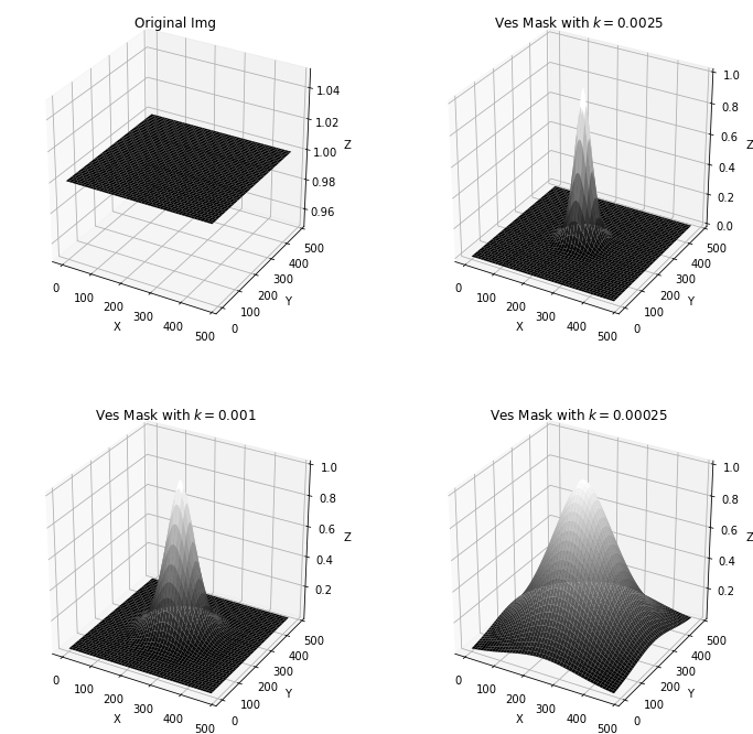
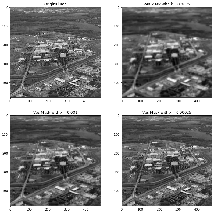
湍流模糊
Hufnagel and Stanley[1964]根据大气湍流的物理特性提出了一个退化模型,其通式为:
\[H(u,v) = e^{-k{(u^2+v^2)}^{5/6}}\]
式中,\(k\)是与湍流性质有关的常熟。除了指数为\(5/6\)之外,该式与高斯低通极其相似。
实现:
1
2
3
4
5
6
7
8
9
10
11
12
13
14
15
16
17
18
19
20
21
22
23
24
25
26
27
28
29
30
31
32
33
34
35
36
37
38
39
40
41
42
43
44
45
46
47
48
49
| def getVesMask(mask_shape,k):
rows,cols = mask_shape[0],mask_shape[1]
crow = rows/2
ccol = cols/2
mask = np.zeros((rows,cols))
for i in range(rows):
for j in range(cols):
dis = (i-crow)**2 + (j-ccol)**2
mask[i,j] = np.exp(-k*(dis**(5/6)))
return mask
def getVesFilterPassImg(input_img : np.array, k , size = None):
f_img = np.fft.fft2(input_img , s = size)
shift_img = np.fft.fftshift(f_img)
mask_shift_img = getVesMask(f_img.shape,k)
new_shift_img = mask_shift_img*shift_img
new_manitude_img = 20*np.log(np.abs(new_shift_img+eps))
new_f_img = np.fft.ifftshift(new_shift_img)
new_img = np.fft.ifft2(new_f_img)
new_img = np.abs(new_img)
return new_img
mask_shape = (480,480)
k = [0,0.0025,0.001,0.00025]
plt.figure(figsize=(12,12))
ax = [plt.subplot(221,projection = "3d"),plt.subplot(222,projection = "3d"),plt.subplot(223,projection = "3d"),plt.subplot(224,projection = "3d")]
for i in range(4):
if i == 0:
drawPerspective(ax[i],np.ones(mask_shape),title ="Original Img",cmap = "gray")
else:
myfilter = getVesMask(mask_shape,k[i])
drawPerspective(ax[i],myfilter,title = f"Ves Mask with $k={k[i]}$", cmap = "gray")
plt.show()
test_img = cv2.imread("./5_3Photo/Fig0525(a).tif",0)
plt.figure(figsize=(12,12))
ax = [plt.subplot(221),plt.subplot(222),plt.subplot(223),plt.subplot(224)]
for i in range(4):
if i == 0:
ax[i].imshow(test_img,cmap = "gray")
ax[i].set_title("Original Img")
else:
out_img = getVesFilterPassImg(test_img,k[i])
ax[i].imshow(out_img,cmap = "gray")
ax[i].set_title(f"Ves Mask with $k={k[i]}$")
|
 png
png
 png
png
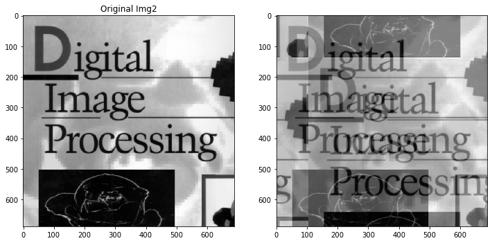
运动模糊
是从基本原理开始推导的一个数学模型,光学成像图像获取时被被图像与传感器之间的均匀线性运动模糊了,最终\(g(x,y)\)反映为\(f(x,y)\)不同时间间隔内瞬时曝光量叠加形成的,(空间域)数学表达为:
\[g(x,y) = \int_0^{T}{ f [x-x_0(t),y-y_0(t)] } \mathrm{d}t\]
频率域中的操作,应用傅里叶变换,中间省略,最后根据\(F(u,v)\)与\(t\)无关得出,我们想要的频率域退化函数表达:
\[H(u,v) = \int_0^T {e^{-j2\pi[ux_0(t)+vy_0(t)]}} \mathrm{d}t\]
满足 x,y 方向做匀速直线运动\(x_0(t) = at/T\)和\(y_0(t) = bt/T\),则退化函数可以直接由上式得。
\[H(u,v) = \dfrac{T}{\pi (ua+vb)} sin[\pi(ua+vb)] e^{-j\pi[ua+vb]}\]
那么我们用\((u,v)\)对该式取样,就可以生成一个离散滤波器,我的实现是(这个实现 bug 了):
1
2
3
4
5
6
7
8
9
10
11
12
13
14
15
16
17
18
19
20
21
22
23
24
25
26
27
28
29
30
31
32
33
34
35
36
37
38
39
| def getMoveMask(mask_shape,param_a,param_b,param_T):
rows,cols = mask_shape[0],mask_shape[1]
crow = rows/2
ccol = cols/2
mask = np.zeros((rows,cols), dtype = np.complex)
for i in range(rows):
for j in range(cols):
if i == 0 and j== 0:
continue
else:
temp = i*param_a+j*param_b
temp2 = np.exp(np.complex(0,-np.pi*temp))
mask[i,j] = temp2*np.sin(np.pi*temp)*param_T/(np.pi*temp)
return mask
def getMoveFilterPassImg(input_img : np.array, a,b,T , size = None):
f_img = np.fft.fft2(input_img , s = size)
shift_img = np.fft.fftshift(f_img)
mask_shift_img = getMoveMask(f_img.shape,a,b,T)
new_shift_img = mask_shift_img*shift_img
new_manitude_img = 20*np.log(np.abs(new_shift_img+eps))
new_f_img = np.fft.ifftshift(new_shift_img)
new_img = np.fft.ifft2(new_f_img)
new_img = np.abs(new_img)
return new_img,new_manitude_img
test_img = cv2.imread("./5_3Photo/Fig0526.tif",0)
a = 0.2
b = 0.15
T = 1
plt.figure(figsize=(12,6))
ax1 = plt.subplot(121)
ax2 = plt.subplot(122)
ax1.imshow(test_img,cmap = "gray")
ax1.set_title("Original Img2")
out_img,test = getMoveFilterPassImg(test_img,a,b,T)
ax2.imshow(out_img,cmap="gray")
plt.show()
|
 png
png
1
2
3
4
5
6
7
8
9
10
11
12
13
14
15
16
17
18
19
20
21
22
23
24
25
26
27
28
29
30
31
32
33
34
35
36
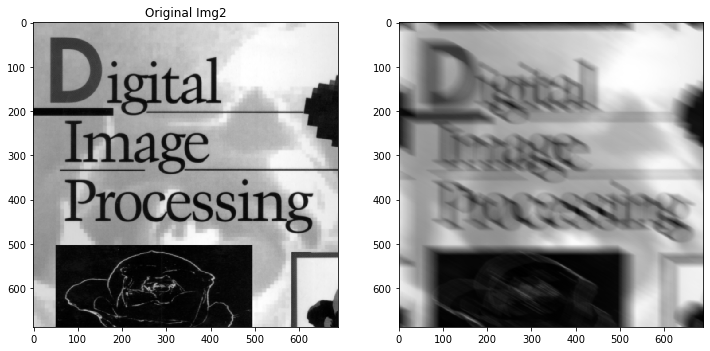
| def getMotionMask(mask_shape,param_len,param_theta):
rows,cols = mask_shape[0],mask_shape[1]
crow = (rows-1)/2
ccol = (cols-1)/2
mask = np.zeros((rows,cols))
sin_val = np.sin(param_theta*np.pi/180)
cos_val = np.cos(param_theta*np.pi/180)
for i in range(param_len):
x_offset = round(sin_val*i)
y_offset = round(cos_val*i)
mask[int(crow+x_offset),int(ccol+y_offset)] =1
mask = mask/mask.sum()
return np.fft.fft2(mask)
def getMotionFilterPassImg(input_img : np.array, l,t , size = None):
f_img = np.fft.fft2(input_img , s = size)
mask_img = getMotionMask(f_img.shape,l,t)
new_img = f_img*mask_img
new_img = np.fft.ifft2(new_img)
output_img = np.fft.ifftshift(new_img)
output_img = np.abs(output_img)
return output_img
test_img = cv2.imread("./5_3Photo/Fig0526.tif",0)
l = 50
t = 30
plt.figure(figsize=(12,6))
ax1 = plt.subplot(121)
ax2 = plt.subplot(122)
ax1.imshow(test_img,cmap = "gray")
ax1.set_title("Original Img2")
out_img = getMotionFilterPassImg(test_img,l,t)
ax2.imshow(out_img,cmap="gray")
plt.show()
|
 png
png
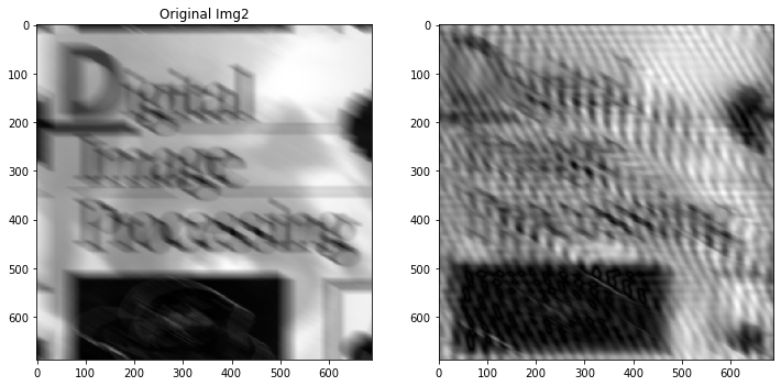
逆滤波
退化函数已给出,或者由上面退化函数的估计方法获得后,最简单的复原方法是直接做逆滤波,即:
\[\hat{F}(u,v) = \dfrac{G(u,v)}{H(u,v)}\]
然而根据前述我们知道,在噪声的影响下,\(\hat{F}(u,v)\)和\(F(u,v)\)仍有差别,即
\[\hat{F}(u,v) = F(u,v) \dfrac{N(u,v)}{H(u,v)}\]
这个式子两点启发:
- 知道退化函数也不能完全复原未退化图像,因为噪声函数未知。
- 如果退化函数是零或是非常小的之,那么噪声影响会被放大
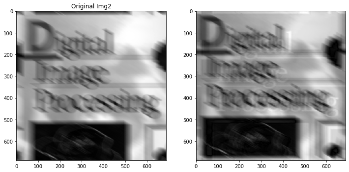
最小均方误差(维纳)滤波
实际上维纳滤波是在这里是相对逆滤波来说的,而并非指特别的滤波函数,且不仅应用在运动模糊滤波中。
\[\hat{F}(u,v) =[\dfrac{1}{H(u,v)} \dfrac{ {|H(u,v)|}^2 }{ {|H(u,v)|}^2+ S_{\eta}(u,v)/S_f(u,v) }] G(u,v)\]
\(S_{\eta}(u,v)\)为噪声的功率谱而\(S_f(u,v)\)是未退化图像的功率谱,比值为噪信比。而由于谱\({|N(u,v)|}^2\)是一个常数,这大大简化了处理。我们常用下面的表达式来近似。
\[\hat{F}(u,v) =[\dfrac{1}{H(u,v)} \dfrac{ {|H(u,v)|}^2 }{ {|H(u,v)|}^2+ K }] G(u,v)\]
1
2
3
4
5
6
7
8
9
10
11
12
13
14
15
16
17
18
19
20
21
22
23
24
25
26
27
28
29
30
31
32
33
34
35
36
37
38
39
40
41
42
43
44
45
46
47
48
49
50
51
52
| def wienerFiltering(input_img, h, NSR ,htype = "frequency"):
assert htype in ("frequency","spatial")
input_img_fft = np.fft.fft2(input_img)
input_img_fft = np.fft.ifftshift(input_img_fft)
if(htype == "spatial"):
h_fft = np.fft.fft2(h)
else :
h_fft = h
h_abs_square = np.abs(h_fft)**2
output_image_fft = np.conj(h_fft) / (h_abs_square + NSR)
output_image = np.fft.ifft2(output_image_fft * input_img_fft)
output_image = np.abs(np.fft.fftshift(output_image))
return output_image
nsr = 0
h = getMotionMask(test_img.shape,l,t)
output_img= getMotionFilterPassImg(test_img,l,t)
plt.figure(figsize=(12,6))
ax1 = plt.subplot(121)
ax2 = plt.subplot(122)
ax1.imshow(output_img,cmap = "gray")
ax1.set_title("Original Img2")
inverse_img = wienerFiltering(out_img,h,nsr,"frequency")
ax2.imshow(inverse_img,cmap="gray")
plt.show()
nsr = 0.01
h = getMotionMask(test_img.shape,l,t)
output_img = getMotionFilterPassImg(test_img,l,t)
plt.figure(figsize=(12,6))
ax1 = plt.subplot(121)
ax2 = plt.subplot(122)
ax1.imshow(output_img,cmap = "gray")
ax1.set_title("Original Img2")
inverse_img = wienerFiltering(out_img,h,nsr,"frequency")
ax2.imshow(inverse_img,cmap="gray")
plt.show()
|
 png
png
 png
png