基本概念
上一篇文章讲了直方图均衡相关内容,从实际应用中我们发现,只能对直方图做均衡操作并不能完全满足我们的需要,有时我们更希望调整概率分布(直方图)为指定形状,这就是直方图匹配。
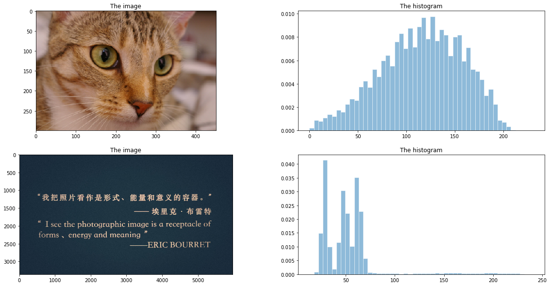
比如下图图一猫咪的直方图较为集中在中间,我们希望它的分布贴近第二幅文字图的分布(集中在暗区域)
 im1
im1
数学基础
从上一篇文章的介绍中我们发现,对于任何图像(\(r\)的概率密度分布),我们都可以通过其累积分布函数将其函数变换到随机变量\(s\),而\(s\)是均匀分布的。那我们反过来想,能否将均匀分布的随机变量逆变换到某个特定的分布呢?
公式推导
设\(r\)为随机变量值域为\([0,255]\),其概率密度函数为\(p_r(r)\)。一函数(变换为):
\[s = T(r) = (L-1) \int_{0}^{r} p_r(m) \mathrm{d}m\]
由上一篇文章我们易知\(s\)服从均匀分布,我们寻找一个\(z\)随机变量符合另一特殊分布\(p_z(z)\),易知存在一函数(变换):
\[s = G(z) = (L-1) \int_{0}^{z} p_z(m) \mathrm{d}m\]
由于\(G(z)\)为累积分布函数,单调,故存在反函数\(G^{-1}(z)\),则有新变换 \(N = G^{-1} \cdot T\),使得\(r\)随机变量经\(N\)变换后符合\(z\)的分布特征。
\[z = G^{-1}(s) = G^{-1}(T(r)) = N(r)\]
由此,我们找到了某值域内求从某一分布随机变量\(r\)变换到指定分布随机变量\(z\)的方法。
个人理解
直方图均衡,均匀分布,实际上在中间做了桥接。
实验效果
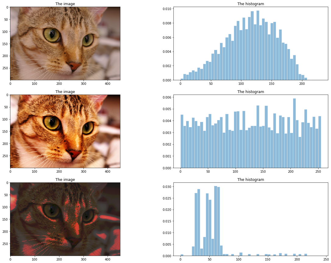
均衡化
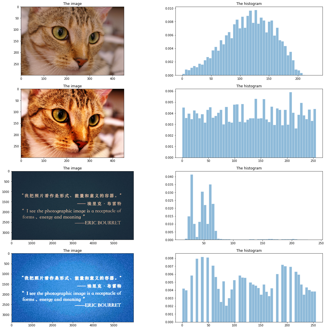
输出两幅图原图以及均衡化后的图片,直方图。
 im1
im1
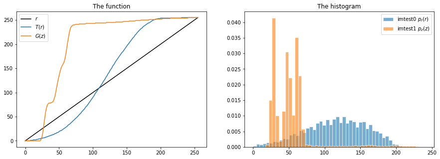
直观对比两图的累积分布函数与直方图
\(T(r)\)表示\(r\)的累积分布函数,本样例中为小猫图像的累积分布函数,图示为淡蓝色曲线。 \(G(z)\)表示为\(z\)的累积分布函数,本样例中为文字图片的累积分布函数,图示为橙黄色曲线。
 im1
im1
求反函数
反函数的计算,并没有按照课本上所说,搜索找最近值,对于一张\(m \times n\)图像,对于每个搜索需要\(O(log(L))\),总复杂度是相乘的关系\(O(MNlog(L))\),而通过一个二重循环实现打表计算则可以优化到\(O(MN)+O(L)\),对于实际图片\(MN\)远大于\(L\),所以这种优化是值得的
1
2
3
4
5
6
| cnt = 0
for i in range(256):
while cnt<=raw_table[i]:
new_table[cnt] = i
cnt+=1
return new_table
|
计算反函数表方便后面对图像进行变换。
1
2
3
| reverse_imtest1_table = GetReverseTable(imtest1_tabel)
match_imtest0_table = reverse_imtest1_table[imtest0_tabel]
match_imtest0 = match_imtest0_table[imtest0]
|
输出结果如下
 im2
im2
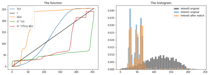
直方图对比表示了 image0,image1,匹配后的 image0 三图,由图可以看出匹配后的 image0 直方图分布已经很贴近 image1 了。
图片效果
(小猫被玩的有点可怜)
 im2
im2
核心代码
图像直方图展示
1
2
3
4
5
6
7
8
9
10
11
12
13
14
15
16
|
def DrawHist(input_img,pic_handle,histogram_handle):
kwargs = dict(bins = 50, histtype='bar', edgecolor = "white",alpha=0.5, density = True)
pic_handle.set_title("The image")
pic_handle.imshow(input_img)
histogram_handle.set_title("The histogram")
histogram_handle.hist(input_img.flatten(),**kwargs)
imtest0 = imageio.imread('imageio:chelsea.png')
imtest1 = GetRGB('./3_3Photo/3.jpg')
plt.figure(figsize=(20,10))
DrawHist(imtest0,plt.subplot(221),plt.subplot(222))
DrawHist(imtest1,plt.subplot(223),plt.subplot(224))
plt.show()
|
直方图匹配
1
2
3
4
5
6
7
8
9
10
|
def GetReverseTable(raw_table):
new_table = np.zeros(256,dtype = np.int64)
cnt = 0
for i in range(256):
    while cnt<=raw_table[i]:
        new_table[cnt] = i
        cnt+=1
return new_table
|
加入反函数输出
1
2
3
4
5
6
7
8
9
10
11
12
13
14
15
16
17
18
19
20
21
22
|
plt.figure(figsize=(15,5))
plotline = plt.subplot(121)
plotline.set_title("The function")
plotline.plot(np.arange(256),imtest0_tabel,label = "$T(r)$")
plotline.plot(np.arange(256),np.arange(256),color = "black",label = "$r$")
plotline.plot(np.arange(256),imtest1_tabel,label = "$G(z)$")
plotline.plot(np.arange(256),reverse_imtest1_table, label = "$G^{-1}(z)$")
plotline.plot(np.arange(256),match_imtest0_table, label= "$G^{-1}(T(r)), N(r)$")
plotline.legend()
kwargs = dict(bins = 50, histtype='bar', edgecolor = "white",alpha=0.5, density = True)
histogram1 = plt.subplot(122)
histogram1.set_title("The histogram")
histogram1.hist(imtest0.flatten(),color = "black",label = "imtest0 original",**kwargs )
histogram1.hist(imtest1.flatten(),label = "imtest1 original",**kwargs)
histogram1.hist(match_imtest0.flatten(),label = "imtest0 after match",**kwargs)
histogram1.legend()
plt.show()
|
完整代码
1
2
3
4
5
6
| import numpy as np
import imageio
import cv2
import matplotlib.pyplot as plt
im = imageio.imread('photo2.jpg')
|
1
2
3
4
5
6
|
def GetRGB(path):
im_BGR = cv2.imread(path,cv2.COLOR_GRAY2RGB)
im = cv2.cvtColor(im_BGR,cv2.COLOR_BGR2RGB)
return im
|
1
2
3
4
5
6
7
8
9
10
11
12
13
14
15
16
|
def DrawHist(input_img,pic_handle,histogram_handle):
kwargs = dict(bins = 50, histtype='bar', edgecolor = "white",alpha=0.5, density = True)
pic_handle.set_title("The image")
pic_handle.imshow(input_img)
histogram_handle.set_title("The histogram")
histogram_handle.hist(input_img.flatten(),**kwargs)
imtest0 = imageio.imread('imageio:chelsea.png')
imtest1 = GetRGB('./3_3Photo/3.jpg')
plt.figure(figsize=(20,10))
DrawHist(imtest0,plt.subplot(221),plt.subplot(222))
DrawHist(imtest1,plt.subplot(223),plt.subplot(224))
plt.show()
|
1
2
3
4
5
6
7
8
9
10
11
12
13
14
15
16
17
18
19
20
21
22
23
24
25
26
27
28
29
30
31
32
33
34
35
36
37
38
39
40
41
42
43
44
45
46
47
48
49
50
51
52
53
54
55
56
57
58
59
60
61
62
63
64
65
66
67
68
69
70
71
72
|
def CaculateHistogram(input_image):
if len(np.shape(input_image)) == 3:
height,width,level = np.shape(input_image)
summ = height*width*level
else :
height,width = np.shape(input_image)
summ = height*width
caculate_num,index_x = GetHistogramArray(input_image)
caculate_num = np.append(caculate_num,1)
sum_num = np.copy(caculate_num)
for i in range(1,256):
sum_num[i] = sum_num[i-1] + sum_num[i]
return summ,caculate_num,sum_num
def GetHistogramArray(image):
return np.histogram(image,np.arange(0,256));
def cumsum(img, bins):
histogram = np.zeros(bins)
for pixel in np.arange(0, bins, 1):
histogram[pixel] += len(img[img==pixel])
return histogram
def HistogramEqualizationLUT(input_image):
size,data,data_sum = CaculateHistogram(input_image)
fxy = lambda x: (255*data_sum[x])//size
table = np.array([fxy(i) for i in range(256)])
lut = lambda x: table[x]
return lut(input_image),table
imtest0_he,imtest0_tabel = HistogramEqualizationLUT(imtest0)
imtest1_he,imtest1_tabel = HistogramEqualizationLUT(imtest1)
plt.figure(figsize=(20,20))
DrawHist(imtest0,plt.subplot(421),plt.subplot(422))
DrawHist(imtest0_he,plt.subplot(423),plt.subplot(424))
DrawHist(imtest1,plt.subplot(425),plt.subplot(426))
DrawHist(imtest1_he,plt.subplot(427),plt.subplot(428))
|
1
2
3
4
5
6
7
8
9
10
11
12
13
14
15
| plt.figure(figsize=(15,5))
plotline = plt.subplot(121)
plotline.set_title("The function")
plotline.plot(np.arange(256),np.arange(256),color = 'black',label = "$r$")
plotline.plot(np.arange(256),imtest0_tabel,label = "$T(r)$")
plotline.plot(np.arange(256),imtest1_tabel,label = "$G(z)$")
plotline.legend()
kwargs = dict(bins = 50, histtype='bar', edgecolor = "white",alpha=0.6, density = True)
histogram = plt.subplot(122)
histogram.set_title("The histogram")
histogram.hist(imtest0.flatten(),**kwargs, label = "imtest0 $p_r(r)$" )
histogram.hist(imtest1.flatten(), **kwargs, label = "imtest1 $p_z(z)$")
histogram.legend()
plt.show()
|
1
2
3
4
5
6
7
8
9
10
11
12
13
14
15
16
|
def GetReverseTable(raw_table):
new_table = np.zeros(256,dtype = np.int64)
cnt = 0
for i in range(256):
while cnt<=raw_table[i]:
new_table[cnt] = i
cnt+=1
return new_table
reverse_imtest1_table = GetReverseTable(imtest1_tabel)
match_imtest0_table = reverse_imtest1_table[imtest0_tabel]
match_imtest0 = match_imtest0_table[imtest0]
|
1
2
3
4
5
6
7
8
9
10
11
12
13
14
15
16
17
18
19
20
21
22
|
plt.figure(figsize=(15,5))
plotline = plt.subplot(121)
plotline.set_title("The function")
plotline.plot(np.arange(256),imtest0_tabel,label = "$T(r)$")
plotline.plot(np.arange(256),np.arange(256),color = "black",label = "$r$")
plotline.plot(np.arange(256),imtest1_tabel,label = "$G(z)$")
plotline.plot(np.arange(256),reverse_imtest1_table, label = "$G^{-1}(z)$")
plotline.plot(np.arange(256),match_imtest0_table, label= "$G^{-1}(T(r)), N(r)$")
plotline.legend()
kwargs = dict(bins = 50, histtype='bar', edgecolor = "white",alpha=0.5, density = True)
histogram1 = plt.subplot(122)
histogram1.set_title("The histogram")
histogram1.hist(imtest0.flatten(),color = "black",label = "imtest0 original",**kwargs )
histogram1.hist(imtest1.flatten(),label = "imtest1 original",**kwargs)
histogram1.hist(match_imtest0.flatten(),label = "imtest0 after match",**kwargs)
histogram1.legend()
plt.show()
|
1
2
3
4
5
6
|
plt.figure(figsize=(20,15))
DrawHist(imtest0,plt.subplot(321),plt.subplot(322))
DrawHist(imtest0_he,plt.subplot(323),plt.subplot(324))
DrawHist(match_imtest0,plt.subplot(325),plt.subplot(326))
plt.show()
|