基本概念
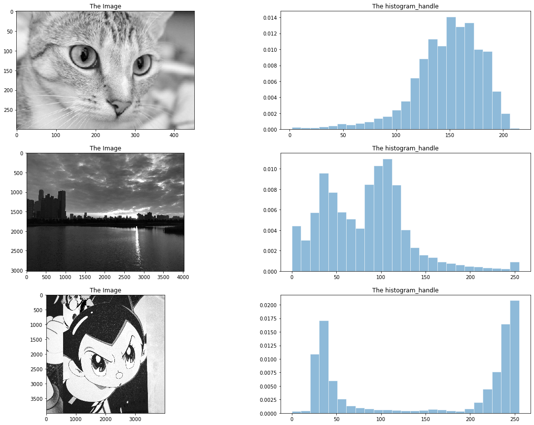
对于一张\(8\)位灰度图像,像素灰度值\(r \in [0,256), r \in Z\),必然满足一特定的概率分布\(p(x)\),直方图可理解为分块显示的概率密度函数。
以下面几图为例(彩色图取 R 通道)
 Sample0
(代码见附录)
由图片可以看出来,图一小猫亮度高的地方更多,所以直方图上显示出在灰度级高端分布更密集,而图二的风景图相反,图三的阿童木则明显亮暗区分较为明显,所以在直方图上体现为两极化。
在某些情况下,我们希望通过某种函数变换\(s = T(r)\),使变换后的函数概率分布均匀化(或贴近均匀),这就是直方图均衡
概率论基础
根据课本 P74 页,\(p_r(r)\)和\(p_s(s)\)分别表示随机变量\(r\)和\(s\)的概率密度函数,概率论的一个基本结果是,如果\(p_r(r)\)和\(T(r)\)已知且\(s = T(r)\)具备单调性,在感兴趣的值域上是连续且可微的,则变换后的变量\(s\)的概率密度函数可由下面的简单公式得到:
\[p_s(s) = p_r(r) \left| \frac{\mathrm{d}r}{\mathrm{d}s} \right|\]
这个式子怎么推导的呢?实际上我们就是在求一个随机变量函数的概率分布,概率论是学过的,这里回忆一下给出推导。
设\(r\)为随机变量,其概率分布符合\(p_r(r)\),另有一单调的函数(变换)\(s = T(r)\),现在求\(s\)的概率分布,设\(r\)值域均为\([0,L-1]\)。
由分布函数公式
\[F(x) = \int_{0}^{x} p(m) \mathrm{d}m\]
得\(r\)得分布函数
\[F_r(r) = \int_{0}^{r} p_r(m) \mathrm{d}m \]
又因为\(s = T(r)\)为单调函数,存在反函数\(r = T^{-1}(s)\)
\[F_s(s) = F_r(T^{-1}(s)) = \int_{0}^{ T^{-1}(s) } p_r(m) \mathrm{d}m \]
概率密度函数为分布函数的导数
\[p_s(s) = \left| \frac{\mathrm{d} F_s(s)}{\mathrm{d}s} \right|\]
应用链式求导法则
\[p_s(s) = \left| \frac{\mathrm{d}F_s(s)}{\mathrm{d}s} \right|\]
\[p_s(s) = \frac{\mathrm{d}F_r(r)}{\mathrm{d}r} \left| \frac{ \mathrm{d} r}{ \mathrm{d}s} \right|\]
\[p_s(s) = p_r(r) \left| \frac{ \mathrm{d} r}{ \mathrm{d}s} \right|\]
则得到了书本上的公式。
均衡变换
有了上述式子,我们会发现特殊的性质
若\(T(r)\)恰为\(r\)的分布函数,则 \[s = T(r) = \int_{0}^{r} p_r(m) \mathrm{d}m \] \[\frac{\mathrm{d}s}{\mathrm{d}r} = p_r(r)\] \[p_s(s) = p_r(r) \left| \frac{ \mathrm{d} r}{ \mathrm{d}s} \right| = p_r(r) \frac{1}{p_r(r)} = 1\]
则\(s\)为均匀分布\(s \in [0,1]\) 且\(p_s(s)\)值恒为\(1\)
若\(T(r)\)为\(r\)分布函数映射到\([0,L-1]\),则 \[s = T(r) = (L-1) \int_{0}^{r} p_r(m) \mathrm{d}m\] \[p_s(s) = p_r(r) \frac{1}{(L-1) p_r(r)} = \frac{1}{L-1}\] 则\(s\)为均匀分布,且\(p_s(s)=\frac{1}{L-1}\)
这便是我们想要的函数变换,无论\(p_r(r)\)分布如何,经过这种类分布函数的函数变换,得到的\(p_s(s)\)就是一个均匀分布。
三通道混合均衡 vs. 分别均衡
平台的讨论区里留下了一个有趣的问题:对于三通道 RGB 图像,对每个通道均衡后合并的图像有时会产生严重的色彩失真。
我的一点理解:
何为失真
在我们的处理过程中,色彩失真(与实际偏差过大),我们可以简单理解为显色偏向与原图产生较大差异,产生新的偏色甚至反向偏色。
我的实验
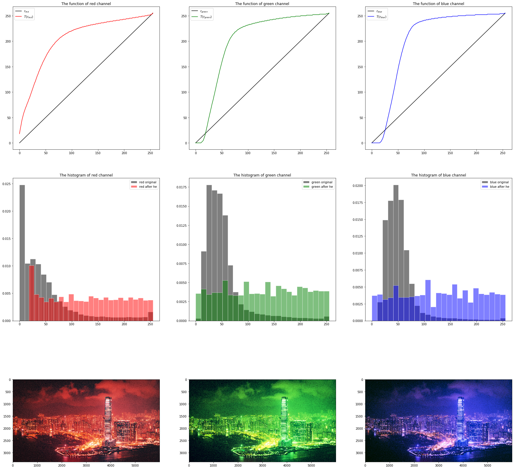
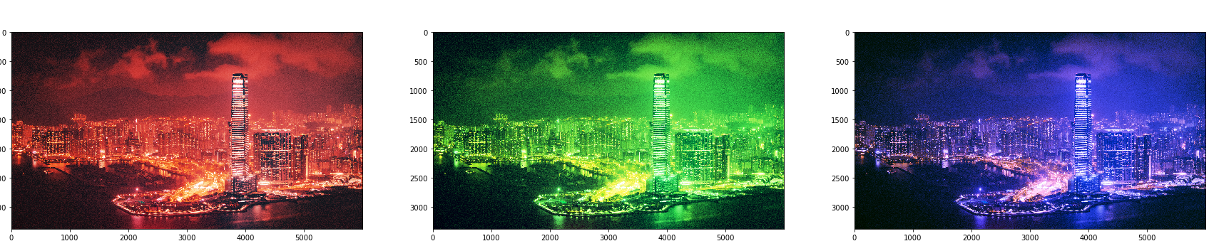
我将一张自己原来拍摄的风景图,R,G,B 三个通道分别进行了直方图均衡,但是没有一同合并,而是与当前未变换的剩下两通道叠加后的图片。
 ThreeChannels1
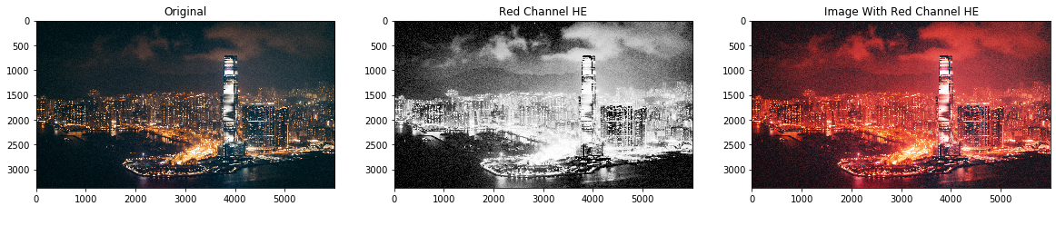
下图是原图,分离的红色通道均衡化图(灰度),均衡化红色通道与原剩余通道叠加图
 ThreeChannels2
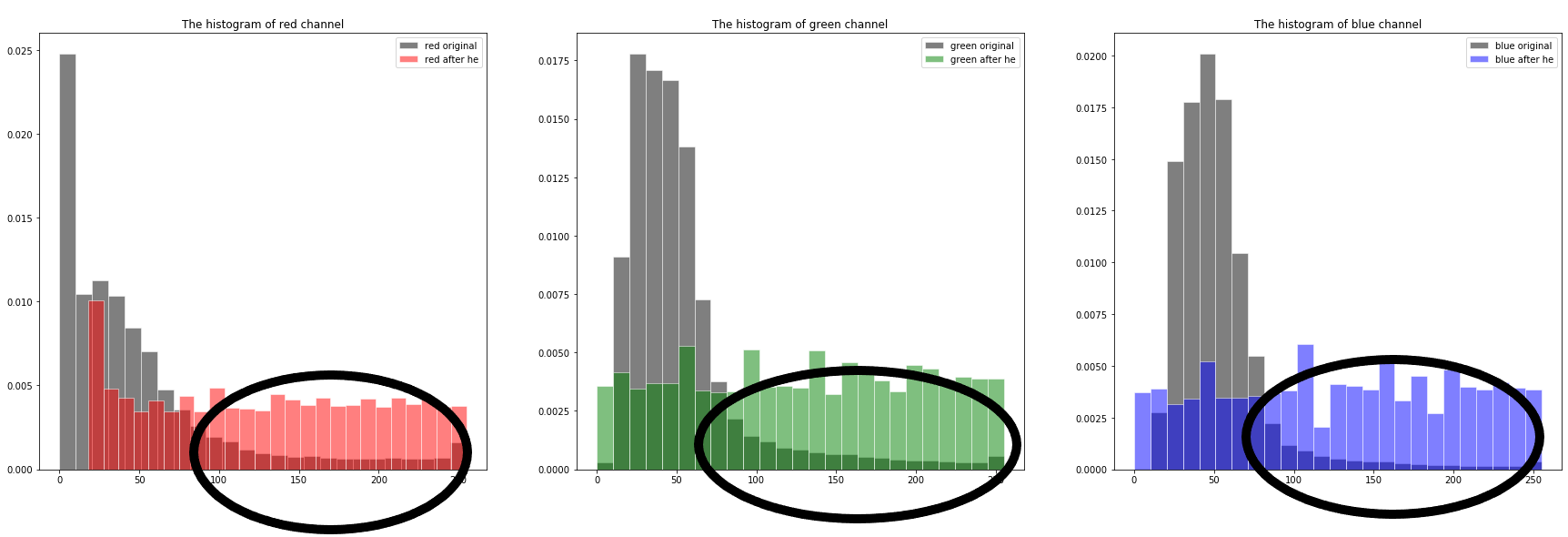
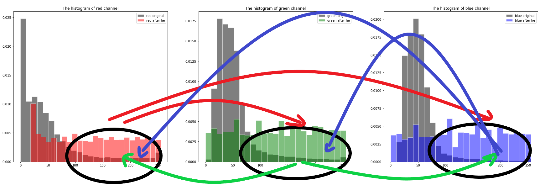
结合原图与与直方图我们不难看出,由于是夜晚照的风景照,整体画面大部分偏暗,所以三个通道的直方图都集中在灰度较低的地方(分布略有偏差)。
当我只均衡一个通道时,该通道直方图中高灰度区域很明显会被提拉上来。
 ThreeChannels3
而相较于其他两通道的中高灰度,被均衡的通道明显概率分布更大。
 ThreeChannels4
所以整体画面会偏向均衡的通道的颜色,如最下面三张合并后的效果所示。
 ThreeChannels5
进一步思考
这种均衡的变换同时也会牺牲掉原本通道高亮的部分,上图蓝色通道的变换最容易看出这种效果。
 ThreeChannels6
均衡化的蓝色通道和剩余两通道合并后的图像中,道路灯光周围较暗的区域更偏向红橙色,这是因为牺牲了原本蓝色在这一灰度范围分布密度的优势,均摊到其他灰度区域后,红绿通道便更加凸显。
进两步思考
无论是从数学推导,还是上述直方图,函数曲线都可以看出来,不同通道颜色的概率密度函数还有累积分布函数都是不同的,则不同通道像素值的相对大小就可能发生改变。
举个例子,若红色通道\(T_{red}(2) = 8\),而蓝色通道\({T_{blue}(5) = 6}\),绿色通道假定不变,则原来像素点\(a = (2,4,5)\) 变换后为\(a' = (8,4,6)\)由偏向蓝色变为偏向红色。
不同通道值对变换后不保序(相同通道由于同一函数单调性确定,必然保序),导致了失真的可能性变大。
因而,若采用三通道合并计算灰度的概率分布然后计算累积分布函数的话,由于使用相同的函数变换,无论是相同通道还是不同通道的两个值\(i\),\(j\),经函数变换后保留其大小关系,如\(i<j \to T(i) < T(j)\)。
这样,虽然在一定程度上牺牲了逐个通道的均衡化效果,但整体上避免了颜色的失真。
进三步思考
实验
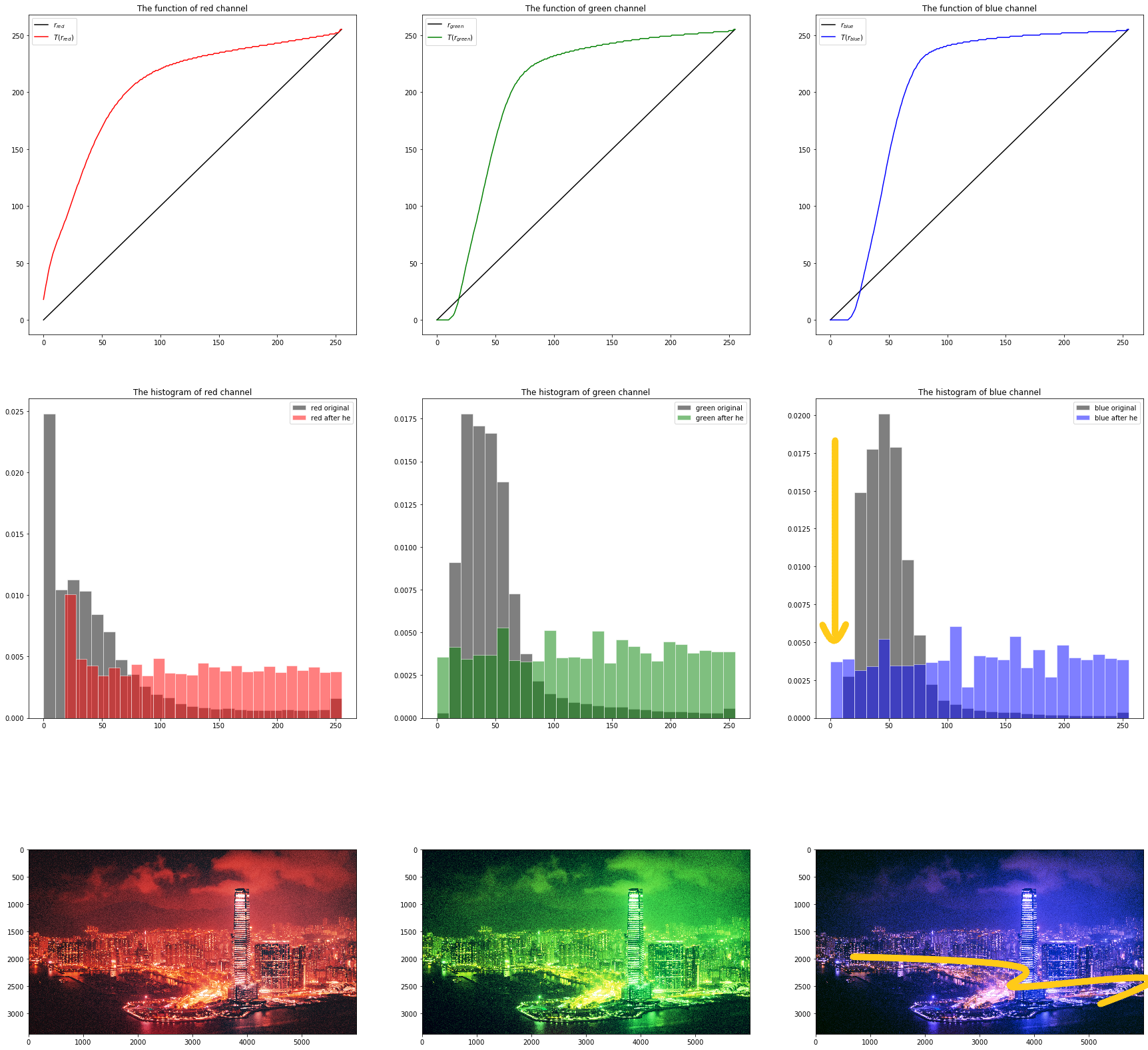
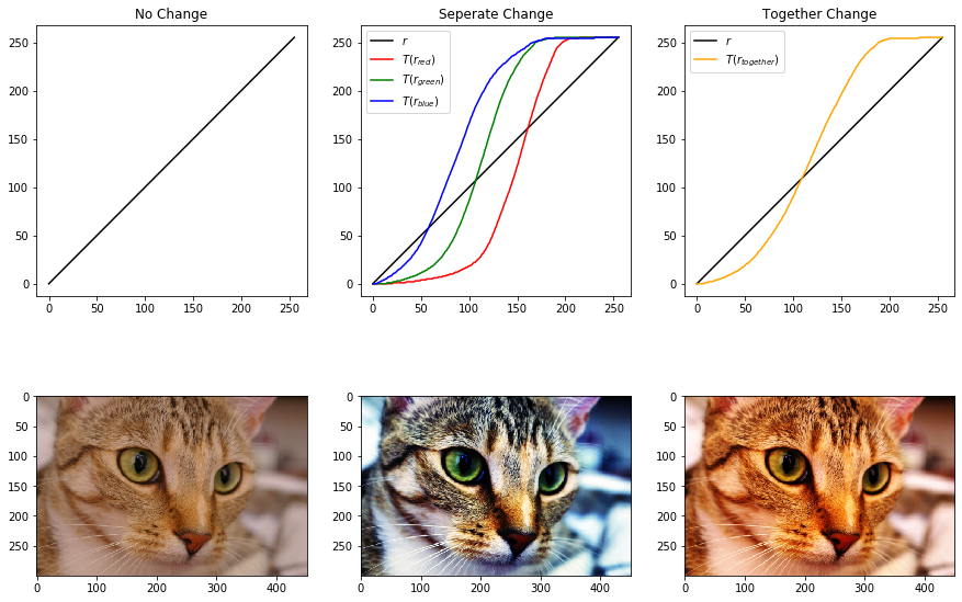
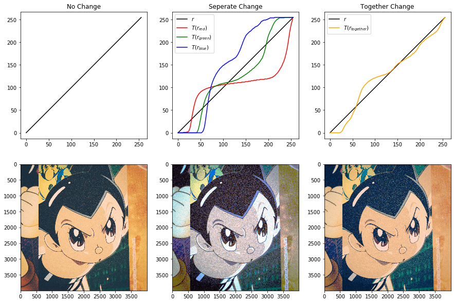
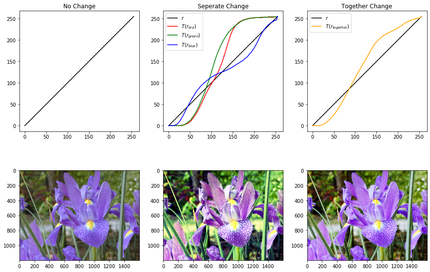
我使用了一些图片做验证,左中右分别对应原图、三通道分别均衡化、整体均衡化的函数曲线和图像。
 Compare0
 Compare1
 Compare2
结论
基本符合预期,整体均衡可以最大程度保留颜色的保真度,三通道虽然在各颜色通道都可以达到均衡效果,但是会造成一定的颜色失真。
核心代码
获取 RGB 三通道图像
需要注意的是,cv2 读取图像为 BGR,需要转换成 RGB。
1
2
3
4
| def GetRGB(path):
im_BGR = cv2.imread(path,cv2.COLOR_GRAY2RGB)
im = cv2.cvtColor(im_BGR,cv2.COLOR_BGR2RGB)
return im
|
获取不同灰度值计数值
通过访问指定位置像素
相同测试环境,耗时 7m9s(最慢)
1
2
3
| for i in range(height):
for j in range(width):
caculate_num[input_image[i][j]] += 1
|
遍历元素
相同测试环境,耗时 14.4s(较慢)
1
2
3
| for line in input_image:
for px in line:
caculate_num[px] +=1
|
向量化比较
相同测试环境,耗时小于 10s(较快)
解释加速原理,img==pixel 得到一个 bool 数组,而 img[]则取出数组为真值的 index 数组,然后就可以用 len()计数了。比较产生 bool 数组是向量操作,底层优化,所以加速效果明显。
1
2
3
4
5
6
7
8
| def cumsum(img, bins):
histogram = np.zeros(bins)
for pixel in np.arange(0, bins, 1):
histogram[pixel] += len(img[img==pixel])
return histogram
caculate_num = cumsum(input_image,256)
print(np.shape(caculate_num))
|
调用 np.histogram()的方法
相同测试环境,耗时 644ms(最快)
快的原因不了解,有时间看看源码
1
2
| caculate_num,index_x = np.histogram(input_image,np.arange(0,256))
caculate_num = np.append(caculate_num,1)
|
直方图均衡化
输入三通/单通道图像,返回均衡化后的图像和查找表
1
2
3
4
5
6
7
8
9
10
11
12
13
14
15
16
17
18
19
20
21
22
23
24
25
26
27
28
29
30
31
32
33
| def CaculateHistogram(input_image):
if len(np.shape(input_image)) == 3:
height,width,level = np.shape(input_image)
summ = height*width*level
else :
height,width = np.shape(input_image)
summ = height*width
caculate_num,index_x = np.histogram(input_image,np.arange(0,256))
 caculate_num = np.append(caculate_num,1)
sum_num = np.copy(caculate_num)
for i in range(1,256):
sum_num[i] = sum_num[i-1] + sum_num[i]
return summ,caculate_num,sum_num
def cumsum(img, bins):
histogram = np.zeros(bins)
for pixel in np.arange(0, bins, 1):
histogram[pixel] += len(img[img==pixel])
return histogram
def HistogramEqualizationLUT(input_image):
size,data,data_sum = CaculateHistogram(input_image)
fxy = lambda x: (255*data_sum[x])//size
table = np.array([fxy(i) for i in range(256)])
lut = lambda x: table[x]
return lut(input_image),table
|
注意要用 lambda,不可以直接 input_new = table[input_image]
绘图函数
1
2
3
4
5
6
7
8
9
10
11
12
13
14
15
16
17
18
19
20
21
22
23
24
25
26
27
28
29
30
31
32
33
34
35
36
37
38
39
40
|
def DrawPerChannel(input_img,split_channel : int, channel_color ,plotline = None, histogram = None, pic = None):
input_channel = input_img[:,:,split_channel]
temp_he,temp_table = HistogramEqualizationLUT(input_channel)
if plotline != None:
plotline.set_title("The function of "+channel_color+" channel")
plotline.plot(np.arange(256),np.arange(256),color = "black",label = "$r_{" + channel_color +"}$")
plotline.plot(np.arange(256),temp_table,color = channel_color ,label = "$T(r_{"+ channel_color +"})$")
plotline.legend()
if histogram != None:
kwargs = dict(bins = 25, histtype='bar', edgecolor = "white",alpha=0.5, density = True)
histogram.set_title("The histogram of "+channel_color+" channel")
histogram.hist(input_channel.flatten(), color = "black",**kwargs, label = channel_color +" original")
histogram.hist(temp_he.flatten(), color = channel_color , **kwargs, label = channel_color +" after he")
histogram.legend()
if pic != None:
show_img = input_img.copy()
show_img[:,:,split_channel] = temp_he
pic.imshow(show_img)
def DrawChannelsEqualization(img_with_3channels):
plt.figure(figsize=(30,30))
DrawPerChannel(img_with_3channels,0,"red",plt.subplot(331),plt.subplot(334),plt.subplot(337))
DrawPerChannel(img_with_3channels,1,"green",plt.subplot(332),plt.subplot(335),plt.subplot(338))
DrawPerChannel(img_with_3channels,2,"blue",plt.subplot(333),plt.subplot(336),plt.subplot(339))
plt.show()
|
1
2
3
4
5
6
7
8
9
10
11
12
13
14
15
16
17
18
19
20
21
22
23
24
25
26
27
28
29
30
31
|
def DrawCompareEqualization(im_with_3_channel):
together_img,together_table = HistogramEqualizationLUT(im_with_3_channel)
seperate_img = im_with_3_channel.copy()
seperate_table = np.array([together_table,together_table,together_table])
for i in range(3):
seperate_img[:,:,i],seperate_table[i] = HistogramEqualizationLUT(im_with_3_channel[:,:,i])
plt.figure(figsize=(15,10))
plotline0 = plt.subplot(231)
plotline0.set_title("No Change")
plotline0.plot(np.arange(256),np.arange(256),color = "black",label = "$r$")
plotline1 = plt.subplot(232)
plotline1.set_title("Seperate Change")
plotline1.plot(np.arange(256),np.arange(256),color = "black",label = "$r$")
plotline1.plot(np.arange(256),seperate_table[0],color = "red" ,label = "$T(r_{red})$")
plotline1.plot(np.arange(256),seperate_table[1],color = "green" ,label = "$T(r_{green})$")
plotline1.plot(np.arange(256),seperate_table[2],color = "blue" ,label = "$T(r_{blue})$")
plotline1.legend()
plotline2 = plt.subplot(233)
plotline2.set_title("Together Change")
plotline2.plot(np.arange(256),np.arange(256),color = "black",label = "$r$")
plotline2.plot(np.arange(256),together_table,color = "orange" ,label = "$T(r_{together})$")
plotline2.legend()
pic0 = plt.subplot(234)
pic0.imshow(im_with_3_channel)
pic1 = plt.subplot(235)
pic1.imshow(seperate_img)
pic2 = plt.subplot(236)
pic2.imshow(together_img)
plt.show()
|
完整代码
1
2
3
4
| import numpy as np
import cv2
import imageio
import matplotlib.pyplot as plt
|
1
2
3
4
5
6
| def GetRGB(path):
im_BGR = cv2.imread(path,cv2.COLOR_GRAY2RGB)
im = cv2.cvtColor(im_BGR,cv2.COLOR_BGR2RGB)
return im
im = GetRGB('./3_2Photo/1.jpg')
|
1
2
3
4
5
6
7
8
9
10
11
12
13
14
15
16
17
18
19
20
21
22
23
24
25
26
27
28
29
30
31
32
33
34
35
36
37
38
39
40
41
42
43
44
45
46
47
48
49
50
51
52
53
54
55
56
57
58
59
60
61
62
63
64
65
66
67
68
69
70
71
72
73
74
75
76
77
78
79
80
81
82
83
84
85
86
87
88
89
90
91
92
93
94
95
96
97
98
99
|
def CaculateHistogram(input_image):
if len(np.shape(input_image)) == 3:
height,width,level = np.shape(input_image)
summ = height*width*level
else :
height,width = np.shape(input_image)
summ = height*width
caculate_num,index_x = GetHistogramArray(input_image)
caculate_num = np.append(caculate_num,1)
sum_num = np.copy(caculate_num)
for i in range(1,256):
sum_num[i] = sum_num[i-1] + sum_num[i]
return summ,caculate_num,sum_num
def GetHistogramArray(image):
return np.histogram(image,np.arange(0,256));
def cumsum(img, bins):
histogram = np.zeros(bins)
for pixel in np.arange(0, bins, 1):
histogram[pixel] += len(img[img==pixel])
return histogram
def HistogramEqualizationLUT(input_image):
size,data,data_sum = CaculateHistogram(input_image)
fxy = lambda x: (255*data_sum[x])//size
table = np.array([fxy(i) for i in range(256)])
lut = lambda x: table[x]
return lut(input_image),table
red_channel_he,red_lut_table = HistogramEqualizationLUT(im[:,:,0])
all_he,lut_table = HistogramEqualizationLUT(im)
plt.figure(figsize=(20,10))
ax1 = plt.subplot(231)
ax1.set_title("Original")
ax1.imshow(im)
ax2 = plt.subplot(232)
ax2.set_title("Red Channel HE")
ax2.imshow(red_channel_he, cmap = 'gray')
new_im = np.copy(im)
new_im[:,:,0] = red_channel_he
ax3 = plt.subplot(233)
ax3.set_title("Image With Red Channel HE")
ax3.imshow(new_im)
ax4 = plt.subplot(234)
ax4.set_title("Original")
ax4.imshow(im)
ax5 = plt.subplot(235)
ax5.set_title("All Channel Together HE")
ax5.imshow(all_he,cmap = "gray")
ax6 = plt.subplot(236)
ax6.set_title("All Channel Together HE")
ax6.imshow(all_he)
plt.show()
|
1
2
3
4
5
6
7
8
9
10
11
12
13
14
15
16
17
18
19
20
21
22
23
24
25
26
27
28
29
30
31
32
33
34
35
36
37
38
39
40
41
42
|
def DrawPerChannel(input_img,split_channel : int, channel_color ,plotline = None, histogram = None, pic = None):
input_channel = input_img[:,:,split_channel]
temp_he,temp_table = HistogramEqualizationLUT(input_channel)
if plotline != None:
plotline.set_title("The function of "+channel_color+" channel")
plotline.plot(np.arange(256),np.arange(256),color = "black",label = "$r_{" + channel_color +"}$")
plotline.plot(np.arange(256),temp_table,color = channel_color ,label = "$T(r_{"+ channel_color +"})$")
plotline.legend()
if histogram != None:
kwargs = dict(bins = 25, histtype='bar', edgecolor = "white",alpha=0.5, density = True)
histogram.set_title("The histogram of "+channel_color+" channel")
histogram.hist(input_channel.flatten(), color = "black",**kwargs, label = channel_color +" original")
histogram.hist(temp_he.flatten(), color = channel_color , **kwargs, label = channel_color +" after he")
histogram.legend()
if pic != None:
show_img = input_img.copy()
show_img[:,:,split_channel] = temp_he
pic.imshow(show_img)
def DrawChannelsEqualization(img_with_3channels):
plt.figure(figsize=(30,30))
DrawPerChannel(img_with_3channels,0,"red",plt.subplot(331),plt.subplot(334),plt.subplot(337))
DrawPerChannel(img_with_3channels,1,"green",plt.subplot(332),plt.subplot(335),plt.subplot(338))
DrawPerChannel(img_with_3channels,2,"blue",plt.subplot(333),plt.subplot(336),plt.subplot(339))
plt.show()
DrawChannelsEqualization(im)
|
1
2
3
4
5
6
7
8
9
10
11
12
13
14
15
16
17
18
19
20
21
22
23
24
25
26
27
28
29
30
31
32
33
|
def DrawCompareEqualization(im_with_3_channel):
together_img,together_table = HistogramEqualizationLUT(im_with_3_channel)
seperate_img = im_with_3_channel.copy()
seperate_table = np.array([together_table,together_table,together_table])
for i in range(3):
seperate_img[:,:,i],seperate_table[i] = HistogramEqualizationLUT(im_with_3_channel[:,:,i])
plt.figure(figsize=(15,10))
plotline0 = plt.subplot(231)
plotline0.set_title("No Change")
plotline0.plot(np.arange(256),np.arange(256),color = "black",label = "$r$")
plotline1 = plt.subplot(232)
plotline1.set_title("Seperate Change")
plotline1.plot(np.arange(256),np.arange(256),color = "black",label = "$r$")
plotline1.plot(np.arange(256),seperate_table[0],color = "red" ,label = "$T(r_{red})$")
plotline1.plot(np.arange(256),seperate_table[1],color = "green" ,label = "$T(r_{green})$")
plotline1.plot(np.arange(256),seperate_table[2],color = "blue" ,label = "$T(r_{blue})$")
plotline1.legend()
plotline2 = plt.subplot(233)
plotline2.set_title("Together Change")
plotline2.plot(np.arange(256),np.arange(256),color = "black",label = "$r$")
plotline2.plot(np.arange(256),together_table,color = "orange" ,label = "$T(r_{together})$")
plotline2.legend()
pic0 = plt.subplot(234)
pic0.imshow(im_with_3_channel)
pic1 = plt.subplot(235)
pic1.imshow(seperate_img)
pic2 = plt.subplot(236)
pic2.imshow(together_img)
plt.show()
DrawCompareEqualization(im)
|
1
2
3
4
5
6
7
8
9
10
11
|
imtest1 = imageio.imread('imageio:chelsea.png')
imtest2 = GetRGB('./3_2Photo/2.jpg')
imtest3 = GetRGB('./3_2Photo/3.jpg')
imtest4 = GetRGB('./3_2Photo/4.tif')
DrawCompareEqualization(imtest1)
DrawCompareEqualization(imtest3)
DrawCompareEqualization(imtest4)
|
1
2
3
4
5
6
7
8
9
10
11
12
13
14
|
def DrawHist(input_img,pic_handle,histogram_handle):
kwargs = dict(bins = 25, histtype='bar', edgecolor = "white",alpha=0.5, density = True)
pic_handle.set_title("The Image")
pic_handle.imshow(input_img,cmap = "gray")
histogram_handle.set_title("The histogram_handle")
histogram_handle.hist(input_img.flatten(),**kwargs)
plt.figure(figsize=(20,15))
DrawHist(imtest1[:,:,0],plt.subplot(321),plt.subplot(322))
DrawHist(imtest2[:,:,0],plt.subplot(323),plt.subplot(324))
DrawHist(imtest3[:,:,0],plt.subplot(325),plt.subplot(326))
plt.show()
|