数字图像处理——频率域平滑锐化图像常用滤波器
频率域滤波器
本文主要是动手实现一些常见的滤波器,并展示其频率域和空间域图像。
这里介绍的常见滤波器为:(高通/低通)理想滤波、布特沃斯滤波器和高斯滤波器,根据书本 P169 页,他们的区别与联系如下:
这三种滤波器涵盖了从非常急剧(理想)的滤波到非常平滑(高斯)的滤波范围。布特沃斯滤波器有一个参数,它成为滤波器的“阶数”。当阶数较高时,布特沃斯滤波器接近于理想滤波器。对于较低的阶数值,布特沃斯滤波器更像高斯滤波器。这样,布特沃斯滤波器可视为两种“极端”滤波器的过渡。
为了方便后续实验,对一些辅助代码模块化编写,主要以可视化部分为主,见文末附录部分。
理想滤波器
所谓"理想"是指无法通过硬件实现的硬截断
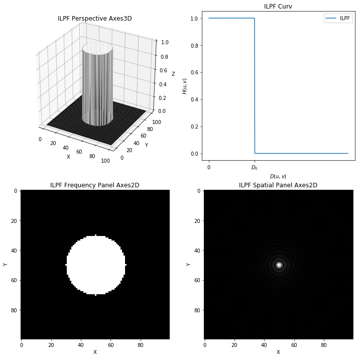
理想低通滤波器 ILPF
在圆外“阻断”所有频率,而在圆内无衰减的通过所有频率,这种二维低通滤波器称为理想低通滤波器(ILPF),由下面的函数确定
\[ H_{ILPF}(u,v) = \left \{ \begin{aligned} 1, & D(u,v) \le D_0 \\ 0, & D(u,b) > D_0 \end{aligned} \right. \]
其中\(D_0\)是一个正常数,\(D(u,v)\)表示频率域中的点\((u,v)\)距离频率域中心\((\frac{P}{2},\frac{Q}{2})\)的距离。
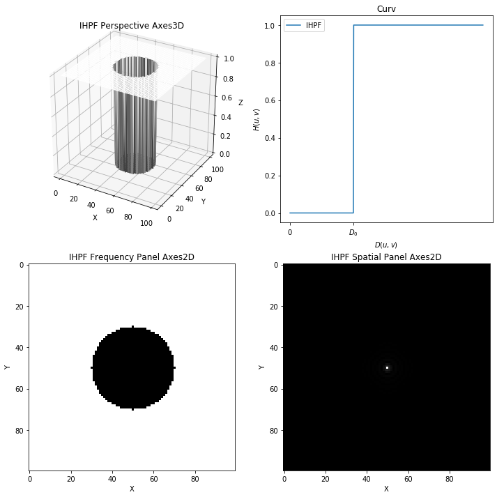
理想高通滤波器 IHPF
与低通类似,高通是将阈值的圆内“阻断”所有频率,而在圆外无衰减的通过所有频率,描述如下
\[ H_{IHPF}(u,v) = \left \{ \begin{aligned} 0, & D(u,v) \le D_0 \\ 1, & D(u,b) > D_0 \end{aligned} \right. \]
代码实现
代码实现低通滤波器并展示其频率域透视图、频率域图像显示、空间域图像显示和径向剖面图。
1 | |
理想低通 ILPF 结果四图
理想高通 IHPF 结果四图
布特沃斯滤波器
可通过硬件实现,可以通过阶数进行控制,一些资料中又称之为“巴特沃斯滤波器”。
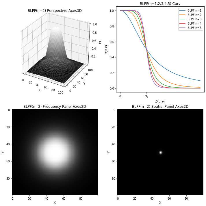
布特沃斯低通滤波器 BLPF
截止频率位于距原点\(D_0\)的\(n\)阶布特沃斯滤波器(BLPF)的传递函数定义为:
\[H_{BLPF}(u,v) = \dfrac{1}{ 1 + {[ \dfrac {D(u,v)}{D_0} ]}^{2n} }\]
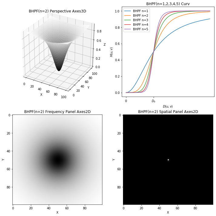
布特沃斯高通滤波器 BHPF
对应的传递函数定义为:
\[H_{BHPF}(u,v) = \dfrac{1}{ 1 + {[ \dfrac {D_0}{D_(u,v)} ]}^{2n} }\]
(分母分子颠倒)
两式中\(n\)对应了即阶参数,下面的代码给出巴特沃斯滤波器的实现,其频率域透视图、频率域图像显示、空间域图像显示和径向剖面图,曲线图绘制出不同阶下的取值。
代码实现
1 | |
布特沃斯低通 BLPF 结果四图
布特沃斯高通 BHPF 结果四图
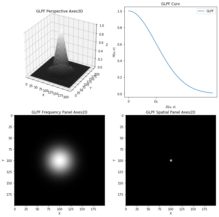
高斯低通滤波器 GLPF
高斯低通滤波器二维形式由下式给处:
\[H_{GLPF}(u,v) = e^{\dfrac{-D^2(u,v)}{2 \sigma^2}}\]
\(\sigma\)描述了中心的扩散速度,和其他滤波器描述式统一,通过令\(\sigma = D_0\),可以用表示其他滤波器的方法表示高斯滤波器。
\[H_{GLPF}(u,v) = e^{\dfrac{-D^2(u,v)}{2 D_0^2}}\]
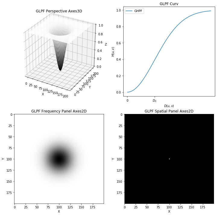
高斯高通滤波器 GHPF
如下:
\[H_{GHPF}(u,v) =1 - e^{\dfrac{-D^2(u,v)}{2 D_0^2}}\]
代码实现
1 | |
高斯低通 GLPF 结果四图
高斯高通 GHPF 结果四图
总结
在规定滤波器为 100x100,阈值为 20 时,可以明显观察到,理想滤波器->高阶布特沃斯滤波器->低阶布特沃斯滤波器->高斯滤波器,可以由函数 Curv 看出对应的过渡。
我们同时也发现理想滤波器确实会存在振铃特性,这个将在后面的文章中再做分析学习。
附录
辅助代码
1 | |
绘制三维透视图
1 | |
绘制平面图
1 | |
绘制曲线图
1 | |
频率域转空间域
1 | |
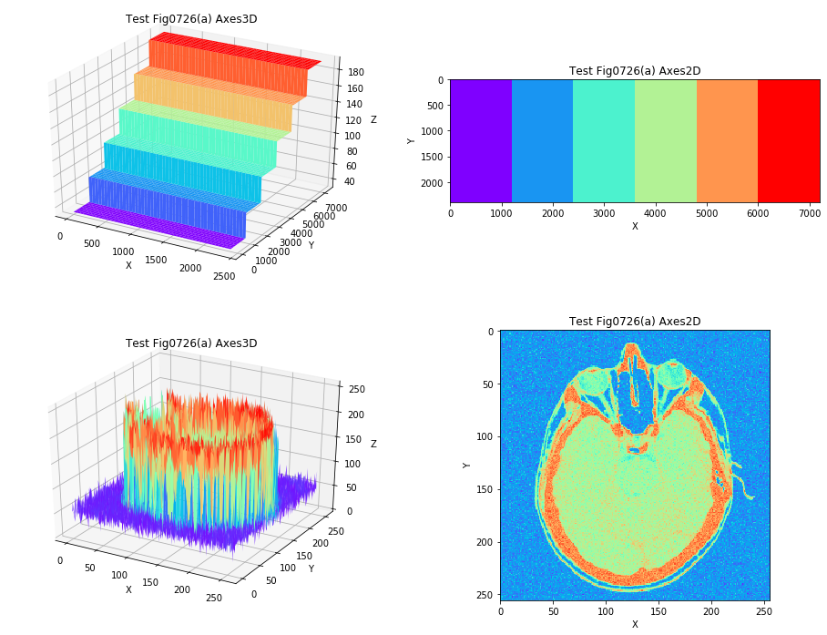
对三维透视可视化代码进行测试
1 | |
测试结果
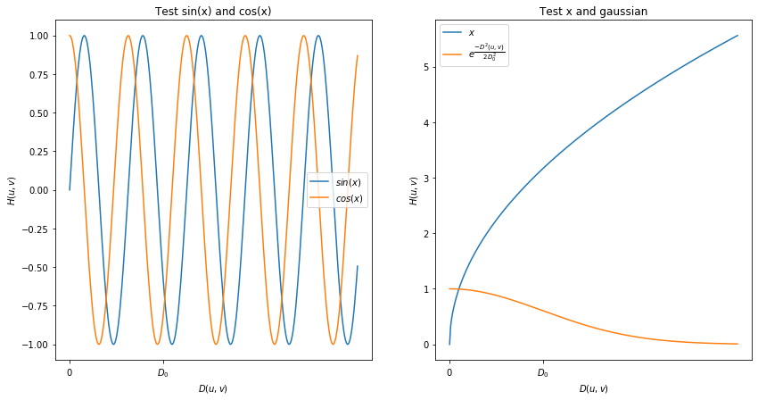
对绘制函数曲线代码进行测试
1 | |
测试结果
本博客所有文章除特别声明外,均采用 CC BY-SA 4.0 协议 ,转载请注明出处!